%sql postgresql://dsi_student:gastudents@dsi.c20gkj5cvu3l.us-east-1.rds.amazonaws.com/titanic
u'Connected: dsi_student@titanic'
import pandas as pd
import numpy as np
%matplotlib inline
import matplotlib.pyplot as plt
%%sql

select * from train limit 5;
| index |
PassengerId |
Survived |
Pclass |
Name |
Sex |
Age |
SibSp |
Parch |
Ticket |
Fare |
Cabin |
Embarked |
| 0 |
1 |
0 |
3 |
Braund, Mr. Owen Harris |
male |
22.0 |
1 |
0 |
A/5 21171 |
7.25 |
None |
S |
| 1 |
2 |
1 |
1 |
Cumings, Mrs. John Bradley (Florence Briggs Thayer) |
female |
38.0 |
1 |
0 |
PC 17599 |
71.2833 |
C85 |
C |
| 2 |
3 |
1 |
3 |
Heikkinen, Miss. Laina |
female |
26.0 |
0 |
0 |
STON/O2. 3101282 |
7.925 |
None |
S |
| 3 |
4 |
1 |
1 |
Futrelle, Mrs. Jacques Heath (Lily May Peel) |
female |
35.0 |
1 |
0 |
113803 |
53.1 |
C123 |
S |
| 4 |
5 |
0 |
3 |
Allen, Mr. William Henry |
male |
35.0 |
0 |
0 |
373450 |
8.05 |
None |
S |
titanic_train = %%sql select * from train;
titanic_df = titanic_train.DataFrame()
|
index |
PassengerId |
Survived |
Pclass |
Name |
Sex |
Age |
SibSp |
Parch |
Ticket |
Fare |
Cabin |
Embarked |
| 0 |
0 |
1 |
0 |
3 |
Braund, Mr. Owen Harris |
male |
22.0 |
1 |
0 |
A/5 21171 |
7.2500 |
None |
S |
| 1 |
1 |
2 |
1 |
1 |
Cumings, Mrs. John Bradley (Florence Briggs Th... |
female |
38.0 |
1 |
0 |
PC 17599 |
71.2833 |
C85 |
C |
| 2 |
2 |
3 |
1 |
3 |
Heikkinen, Miss. Laina |
female |
26.0 |
0 |
0 |
STON/O2. 3101282 |
7.9250 |
None |
S |
| 3 |
3 |
4 |
1 |
1 |
Futrelle, Mrs. Jacques Heath (Lily May Peel) |
female |
35.0 |
1 |
0 |
113803 |
53.1000 |
C123 |
S |
| 4 |
4 |
5 |
0 |
3 |
Allen, Mr. William Henry |
male |
35.0 |
0 |
0 |
373450 |
8.0500 |
None |
S |
# titanic_df[0:50]
titanic_df[titanic_df['Cabin'] == 'G6']
|
index |
PassengerId |
Survived |
Pclass |
Name |
Sex |
Age |
SibSp |
Parch |
Ticket |
Fare |
Cabin |
Embarked |
| 10 |
10 |
11 |
1 |
3 |
Sandstrom, Miss. Marguerite Rut |
female |
4.0 |
1 |
1 |
PP 9549 |
16.7000 |
G6 |
S |
| 205 |
205 |
206 |
0 |
3 |
Strom, Miss. Telma Matilda |
female |
2.0 |
0 |
1 |
347054 |
10.4625 |
G6 |
S |
| 251 |
251 |
252 |
0 |
3 |
Strom, Mrs. Wilhelm (Elna Matilda Persson) |
female |
29.0 |
1 |
1 |
347054 |
10.4625 |
G6 |
S |
| 394 |
394 |
395 |
1 |
3 |
Sandstrom, Mrs. Hjalmar (Agnes Charlotta Bengt... |
female |
24.0 |
0 |
2 |
PP 9549 |
16.7000 |
G6 |
S |
titanic_df[titanic_df['Ticket'] == 'PP 9549']
|
index |
PassengerId |
Survived |
Pclass |
Name |
Sex |
Age |
SibSp |
Parch |
Ticket |
Fare |
Cabin |
Embarked |
| 10 |
10 |
11 |
1 |
3 |
Sandstrom, Miss. Marguerite Rut |
female |
4.0 |
1 |
1 |
PP 9549 |
16.7 |
G6 |
S |
| 394 |
394 |
395 |
1 |
3 |
Sandstrom, Mrs. Hjalmar (Agnes Charlotta Bengt... |
female |
24.0 |
0 |
2 |
PP 9549 |
16.7 |
G6 |
S |
#titanic_df[titanic_df['Cabin'] == re.compile]
titanic_df[titanic_df['Name'].str.contains("Sandstrom")]
|
index |
PassengerId |
Survived |
Pclass |
Name |
Sex |
Age |
SibSp |
Parch |
Ticket |
Fare |
Cabin |
Embarked |
| 10 |
10 |
11 |
1 |
3 |
Sandstrom, Miss. Marguerite Rut |
female |
4.0 |
1 |
1 |
PP 9549 |
16.7 |
G6 |
S |
| 394 |
394 |
395 |
1 |
3 |
Sandstrom, Mrs. Hjalmar (Agnes Charlotta Bengt... |
female |
24.0 |
0 |
2 |
PP 9549 |
16.7 |
G6 |
S |
u'Sandstrom, Mrs. Hjalmar (Agnes Charlotta Bengtsson)'
test = pd.read_csv('test.csv')
test[test['Name'].str.contains("Sandstrom")]
|
PassengerId |
Pclass |
Name |
Sex |
Age |
SibSp |
Parch |
Ticket |
Fare |
Cabin |
Embarked |
| 117 |
1009 |
3 |
Sandstrom, Miss. Beatrice Irene |
female |
1.0 |
1 |
1 |
PP 9549 |
16.7 |
G6 |
S |
dropped = ['index', 'PassengerId']
df = titanic_df.drop(dropped, 1)
|
Survived |
Pclass |
Name |
Sex |
Age |
SibSp |
Parch |
Ticket |
Fare |
Cabin |
Embarked |
| 0 |
0 |
3 |
Braund, Mr. Owen Harris |
male |
22.0 |
1 |
0 |
A/5 21171 |
7.2500 |
None |
S |
| 1 |
1 |
1 |
Cumings, Mrs. John Bradley (Florence Briggs Th... |
female |
38.0 |
1 |
0 |
PC 17599 |
71.2833 |
C85 |
C |
| 2 |
1 |
3 |
Heikkinen, Miss. Laina |
female |
26.0 |
0 |
0 |
STON/O2. 3101282 |
7.9250 |
None |
S |
| 3 |
1 |
1 |
Futrelle, Mrs. Jacques Heath (Lily May Peel) |
female |
35.0 |
1 |
0 |
113803 |
53.1000 |
C123 |
S |
| 4 |
0 |
3 |
Allen, Mr. William Henry |
male |
35.0 |
0 |
0 |
373450 |
8.0500 |
None |
S |
Check for null values
df.Age.isnull().value_counts()
False    714
True     177
Name: Age, dtype: int64
# will need to find a way to impute age, else will use median
df.Embarked.isnull().value_counts()
False    889
True       2
Name: Embarked, dtype: int64
# since only two embarked values are missing will fill with majority class
df.Embarked.value_counts()
S    644
C    168
Q     77
Name: Embarked, dtype: int64
# Check two missing embarked indexes
df[df.Embarked.isnull() == True]
|
Survived |
Pclass |
Name |
Sex |
Age |
SibSp |
Parch |
Ticket |
Fare |
Cabin |
Embarked |
| 61 |
1 |
1 |
Icard, Miss. Amelie |
female |
38.0 |
0 |
0 |
113572 |
80.0 |
B28 |
None |
| 829 |
1 |
1 |
Stone, Mrs. George Nelson (Martha Evelyn) |
female |
62.0 |
0 |
0 |
113572 |
80.0 |
B28 |
None |
# Let's see if the ticket numbers can give us a clue,
# Search for similar ticket numbers with fuzzy wuzzy
from fuzzywuzzy import fuzz
from fuzzywuzzy import process
query = '113572'
choices = df.Ticket

process.extract(query, choices)
[(u'113572', 100),
 (u'113572', 100),
 (u'113792', 83),
 (u'5727', 77),
 (u'11752', 73)]
df[df['Ticket'] == '113792']
|
Survived |
Pclass |
Name |
Sex |
Age |
SibSp |
Parch |
Ticket |
Fare |
Cabin |
Embarked |
| 467 |
0 |
1 |
Smart, Mr. John Montgomery |
male |
56.0 |
0 |
0 |
113792 |
26.55 |
None |
S |
# df[df['Ticket'].str.contains('113')]
df['Embarked'] = df['Embarked'].fillna('S')
df['Embarked'].isnull().value_counts()
False    891
Name: Embarked, dtype: int64
# Check for missing values in Cabin
df.Cabin.isnull().value_counts()
True     687
False    204
Name: Cabin, dtype: int64
# We will not really be able to impute Missing cabins and some passengeres were not assigned a cabin
# so will replace with value for missing
Feature engineering
# Create a family size feature
df['Fsize'] = df['SibSp'] + df['Parch'] + 1
# Pull Titles from Name
import re
def titles(string):
    titles = re.search(' ([A-Za-z]+)\.', string)
    # If the title exists, extract and return it.
    if titles:
        return titles.group(1)
    return ""
# Create a new feature Title, containing the titles of passenger names
df['title'] = df['Name'].apply(titles)
Mr          517
Miss        182
Mrs         125
Master       40
Dr            7
Rev           6
Col           2
Major         2
Mlle          2
Countess      1
Ms            1
Lady          1
Jonkheer      1
Don           1
Mme           1
Capt          1
Sir           1
Name: title, dtype: int64
df['title'][df['title'] == 'Mlle'] = 'Miss'
/anaconda/lib/python2.7/site-packages/ipykernel/__main__.py:1: SettingWithCopyWarning:
A value is trying to be set on a copy of a slice from a DataFrame

See the caveats in the documentation: http://pandas.pydata.org/pandas-docs/stable/indexing.html#indexing-view-versus-copy
  if __name__ == '__main__':
df['title'][df['title'] == 'Countess'] = 'Lady'
/anaconda/lib/python2.7/site-packages/ipykernel/__main__.py:1: SettingWithCopyWarning:
A value is trying to be set on a copy of a slice from a DataFrame

See the caveats in the documentation: http://pandas.pydata.org/pandas-docs/stable/indexing.html#indexing-view-versus-copy
  if __name__ == '__main__':
df['title'][df['title'] == 'Mme'] = 'Ms'
/anaconda/lib/python2.7/site-packages/ipykernel/__main__.py:1: SettingWithCopyWarning:
A value is trying to be set on a copy of a slice from a DataFrame

See the caveats in the documentation: http://pandas.pydata.org/pandas-docs/stable/indexing.html#indexing-view-versus-copy
  if __name__ == '__main__':
male_hon = ['Major', 'Col','Jonkheer','Don','Capt']
for i in male_hon:
    df['title'][df['title'] == i] = 'MHon'
/anaconda/lib/python2.7/site-packages/ipykernel/__main__.py:3: SettingWithCopyWarning:
A value is trying to be set on a copy of a slice from a DataFrame

See the caveats in the documentation: http://pandas.pydata.org/pandas-docs/stable/indexing.html#indexing-view-versus-copy
  app.launch_new_instance()
|
Survived |
Pclass |
Name |
Sex |
Age |
SibSp |
Parch |
Ticket |
Fare |
Cabin |
Embarked |
Fsize |
title |
| 245 |
0 |
1 |
Minahan, Dr. William Edward |
male |
44.0 |
2 |
0 |
19928 |
90.0000 |
C78 |
Q |
3 |
Dr |
| 317 |
0 |
2 |
Moraweck, Dr. Ernest |
male |
54.0 |
0 |
0 |
29011 |
14.0000 |
None |
S |
1 |
Dr |
| 398 |
0 |
2 |
Pain, Dr. Alfred |
male |
23.0 |
0 |
0 |
244278 |
10.5000 |
None |
S |
1 |
Dr |
| 632 |
1 |
1 |
Stahelin-Maeglin, Dr. Max |
male |
32.0 |
0 |
0 |
13214 |
30.5000 |
B50 |
C |
1 |
Dr |
| 660 |
1 |
1 |
Frauenthal, Dr. Henry William |
male |
50.0 |
2 |
0 |
PC 17611 |
133.6500 |
None |
S |
3 |
Dr |
| 766 |
0 |
1 |
Brewe, Dr. Arthur Jackson |
male |
NaN |
0 |
0 |
112379 |
39.6000 |
None |
C |
1 |
Dr |
| 796 |
1 |
1 |
Leader, Dr. Alice (Farnham) |
female |
49.0 |
0 |
0 |
17465 |
25.9292 |
D17 |
S |
1 |
Dr |
Mr        517
Miss      184
Mrs       125
Master     40
MHon        7
Dr          7
Rev         6
Ms          2
Lady        2
Sir         1
Name: title, dtype: int64
# Fill missing cabin values with 'X'
df['Cabin'] = df['Cabin'].fillna('X')
# Create a feature for Deck
# Pull deck from Cabin
def deck(string):
    decks = re.search('[A-Za-z]', string)
    # If the deck exists, extract and return it.
    if decks:
        return decks.group(0)
    return ""
# Create a new feature deck
df['deck'] = df['Cabin'].apply(deck)
|
Survived |
Pclass |
Name |
Sex |
Age |
SibSp |
Parch |
Ticket |
Fare |
Cabin |
Embarked |
Fsize |
title |
deck |
| 0 |
0 |
3 |
Braund, Mr. Owen Harris |
male |
22.0 |
1 |
0 |
A/5 21171 |
7.2500 |
X |
S |
2 |
Mr |
X |
| 1 |
1 |
1 |
Cumings, Mrs. John Bradley (Florence Briggs Th... |
female |
38.0 |
1 |
0 |
PC 17599 |
71.2833 |
C85 |
C |
2 |
Mrs |
C |
| 2 |
1 |
3 |
Heikkinen, Miss. Laina |
female |
26.0 |
0 |
0 |
STON/O2. 3101282 |
7.9250 |
X |
S |
1 |
Miss |
X |
| 3 |
1 |
1 |
Futrelle, Mrs. Jacques Heath (Lily May Peel) |
female |
35.0 |
1 |
0 |
113803 |
53.1000 |
C123 |
S |
2 |
Mrs |
C |
| 4 |
0 |
3 |
Allen, Mr. William Henry |
male |
35.0 |
0 |
0 |
373450 |
8.0500 |
X |
S |
1 |
Mr |
X |
df['deck'][df['Pclass'] == 2].value_counts()
X    168
F      8
D      4
E      4
Name: deck, dtype: int64
# Surname feature, will try using this feature in decision tree models
names = df['Name'].str.split(',')
surnames = []
for i in names:
    surnames.append(i[0])
df['surname'] = surnames
|
Survived |
Pclass |
Name |
Sex |
Age |
SibSp |
Parch |
Ticket |
Fare |
Cabin |
Embarked |
Fsize |
title |
deck |
surname |
| 0 |
0 |
3 |
Braund, Mr. Owen Harris |
male |
22.0 |
1 |
0 |
A/5 21171 |
7.2500 |
X |
S |
2 |
Mr |
X |
Braund |
| 1 |
1 |
1 |
Cumings, Mrs. John Bradley (Florence Briggs Th... |
female |
38.0 |
1 |
0 |
PC 17599 |
71.2833 |
C85 |
C |
2 |
Mrs |
C |
Cumings |
| 2 |
1 |
3 |
Heikkinen, Miss. Laina |
female |
26.0 |
0 |
0 |
STON/O2. 3101282 |
7.9250 |
X |
S |
1 |
Miss |
X |
Heikkinen |
| 3 |
1 |
1 |
Futrelle, Mrs. Jacques Heath (Lily May Peel) |
female |
35.0 |
1 |
0 |
113803 |
53.1000 |
C123 |
S |
2 |
Mrs |
C |
Futrelle |
| 4 |
0 |
3 |
Allen, Mr. William Henry |
male |
35.0 |
0 |
0 |
373450 |
8.0500 |
X |
S |
1 |
Mr |
X |
Allen |
df[["Sex", "Survived"]].groupby(['Sex'], as_index=False).mean()
|
Sex |
Survived |
| 0 |
female |
0.742038 |
| 1 |
male |
0.188908 |
df[["Fsize", "Survived"]].groupby(['Fsize'], as_index=False).mean()
|
Fsize |
Survived |
| 0 |
1 |
0.303538 |
| 1 |
2 |
0.552795 |
| 2 |
3 |
0.578431 |
| 3 |
4 |
0.724138 |
| 4 |
5 |
0.200000 |
| 5 |
6 |
0.136364 |
| 6 |
7 |
0.333333 |
| 7 |
8 |
0.000000 |
| 8 |
11 |
0.000000 |
|
Survived |
Pclass |
Name |
Sex |
Age |
SibSp |
Parch |
Ticket |
Fare |
Cabin |
Embarked |
Fsize |
title |
deck |
surname |
| 159 |
0 |
3 |
Sage, Master. Thomas Henry |
male |
NaN |
8 |
2 |
CA. 2343 |
69.55 |
X |
S |
11 |
Master |
X |
Sage |
| 180 |
0 |
3 |
Sage, Miss. Constance Gladys |
female |
NaN |
8 |
2 |
CA. 2343 |
69.55 |
X |
S |
11 |
Miss |
X |
Sage |
| 201 |
0 |
3 |
Sage, Mr. Frederick |
male |
NaN |
8 |
2 |
CA. 2343 |
69.55 |
X |
S |
11 |
Mr |
X |
Sage |
| 324 |
0 |
3 |
Sage, Mr. George John Jr |
male |
NaN |
8 |
2 |
CA. 2343 |
69.55 |
X |
S |
11 |
Mr |
X |
Sage |
| 792 |
0 |
3 |
Sage, Miss. Stella Anna |
female |
NaN |
8 |
2 |
CA. 2343 |
69.55 |
X |
S |
11 |
Miss |
X |
Sage |
| 846 |
0 |
3 |
Sage, Mr. Douglas Bullen |
male |
NaN |
8 |
2 |
CA. 2343 |
69.55 |
X |
S |
11 |
Mr |
X |
Sage |
| 863 |
0 |
3 |
Sage, Miss. Dorothy Edith "Dolly" |
female |
NaN |
8 |
2 |
CA. 2343 |
69.55 |
X |
S |
11 |
Miss |
X |
Sage |
test[test['Name'].str.contains('Sage')]
|
PassengerId |
Pclass |
Name |
Sex |
Age |
SibSp |
Parch |
Ticket |
Fare |
Cabin |
Embarked |
| 188 |
1080 |
3 |
Sage, Miss. Ada |
female |
NaN |
8 |
2 |
CA. 2343 |
69.55 |
NaN |
S |
| 342 |
1234 |
3 |
Sage, Mr. John George |
male |
NaN |
1 |
9 |
CA. 2343 |
69.55 |
NaN |
S |
| 360 |
1252 |
3 |
Sage, Master. William Henry |
male |
14.5 |
8 |
2 |
CA. 2343 |
69.55 |
NaN |
S |
| 365 |
1257 |
3 |
Sage, Mrs. John (Annie Bullen) |
female |
NaN |
1 |
9 |
CA. 2343 |
69.55 |
NaN |
S |
# It appears the fare column may be fare per ticket and not per passenger
# Will try and address that later if time permits
df[["Parch", "Survived"]].groupby(['Parch'], as_index=False).mean()
|
Parch |
Survived |
| 0 |
0 |
0.343658 |
| 1 |
1 |
0.550847 |
| 2 |
2 |
0.500000 |
| 3 |
3 |
0.600000 |
| 4 |
4 |
0.000000 |
| 5 |
5 |
0.200000 |
| 6 |
6 |
0.000000 |
df[["Pclass", "Survived"]].groupby(['Pclass'], as_index=False).mean()
|
Pclass |
Survived |
| 0 |
1 |
0.629630 |
| 1 |
2 |
0.472826 |
| 2 |
3 |
0.242363 |
df[["Fsize", "Survived"]].groupby(['Fsize'], as_index=False).mean()
|
Fsize |
Survived |
| 0 |
1 |
0.303538 |
| 1 |
2 |
0.552795 |
| 2 |
3 |
0.578431 |
| 3 |
4 |
0.724138 |
| 4 |
5 |
0.200000 |
| 5 |
6 |
0.136364 |
| 6 |
7 |
0.333333 |
| 7 |
8 |
0.000000 |
| 8 |
11 |
0.000000 |
df[df['Ticket'] == 'F.C.C. 13529']
|
Survived |
Pclass |
Name |
Sex |
Age |
SibSp |
Parch |
Ticket |
Fare |
Cabin |
Embarked |
Fsize |
title |
deck |
surname |
| 314 |
0 |
2 |
Hart, Mr. Benjamin |
male |
43.0 |
1 |
1 |
F.C.C. 13529 |
26.25 |
X |
S |
3 |
Mr |
X |
Hart |
| 440 |
1 |
2 |
Hart, Mrs. Benjamin (Esther Ada Bloomfield) |
female |
45.0 |
1 |
1 |
F.C.C. 13529 |
26.25 |
X |
S |
3 |
Mrs |
X |
Hart |
| 535 |
1 |
2 |
Hart, Miss. Eva Miriam |
female |
7.0 |
0 |
2 |
F.C.C. 13529 |
26.25 |
X |
S |
3 |
Miss |
X |
Hart |
pd.pivot_table(df[df['Age'].isnull() == True], index=['Pclass', 'title'], values=['Age'])
|
|
Age |
| Pclass |
title |
|
| 1 |
Dr |
NaN |
| Miss |
NaN |
| Mr |
NaN |
| Mrs |
NaN |
| 2 |
Miss |
NaN |
| Mr |
NaN |
| 3 |
Master |
NaN |
| Miss |
NaN |
| Mr |
NaN |
| Mrs |
NaN |
# Fill missings ages with median for title and pclass
df['Age'].fillna(df.groupby(["title", "Pclass"])["Age"].transform("median"), inplace=True)
df['Age'].isnull().value_counts()
False    891
Name: Age, dtype: int64
df['Age'][df['title'] == 'Dr'][df['Pclass'] == 1]
245    44.0
632    32.0
660    50.0
766    46.5
796    49.0
Name: Age, dtype: float64
df['Age'][df['title'] == 'Dr'][df['Pclass'] == 1].median()
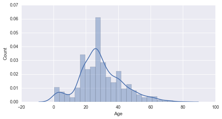
Lets plot some of our features and Determine how to treat them
# Create a list of quantitative data columns
quant = [f for f in df.columns if df.dtypes[f] != 'object']
quant
[u'Survived', u'Pclass', u'Age', u'SibSp', u'Parch', u'Fare', 'Fsize']
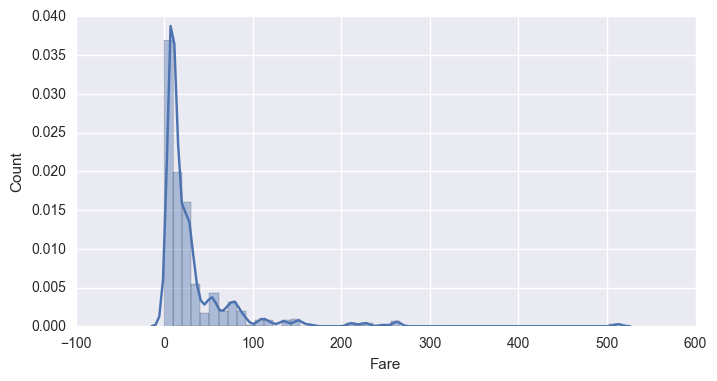
# Plot Histograms of numerical data columns
sns.set(rc={"figure.figsize": (8, 4)})
for i in hists:
    sns.distplot(df[i])
    plt.xlabel(i)
    plt.ylabel('Count')
    plt.show()
|
Survived |
Pclass |
Name |
Sex |
Age |
SibSp |
Parch |
Ticket |
Fare |
Cabin |
Embarked |
Fsize |
title |
deck |
surname |
| 258 |
1 |
1 |
Ward, Miss. Anna |
female |
35.0 |
0 |
0 |
PC 17755 |
512.3292 |
X |
C |
1 |
Miss |
X |
Ward |
| 679 |
1 |
1 |
Cardeza, Mr. Thomas Drake Martinez |
male |
36.0 |
0 |
1 |
PC 17755 |
512.3292 |
B51 B53 B55 |
C |
2 |
Mr |
B |
Cardeza |
| 737 |
1 |
1 |
Lesurer, Mr. Gustave J |
male |
35.0 |
0 |
0 |
PC 17755 |
512.3292 |
B101 |
C |
1 |
Mr |
B |
Lesurer |
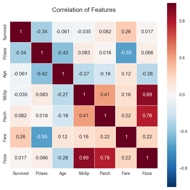
plt.figure(figsize=(8,8))
plt.title('Correlation of Features', y=1.05, size=15)
sns.heatmap(df.corr(),linewidths=0.1,vmax=1.0, square=True, linecolor='white', annot=True)
<matplotlib.axes._subplots.AxesSubplot at 0x1130a55d0>
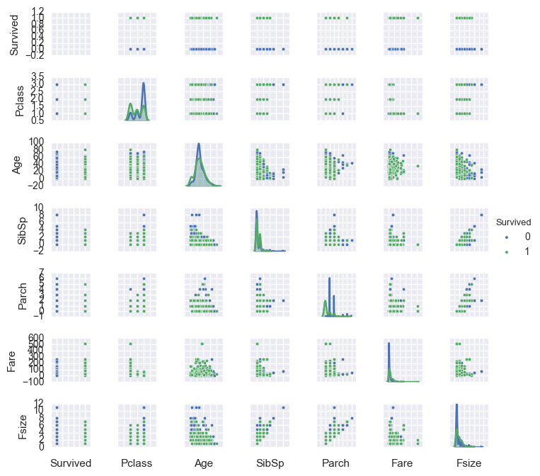
g = sns.pairplot(df[['Survived', 'Pclass', 'Sex', 'Age', 'SibSp','Parch', 'Fare', 'Embarked', 'Fsize', 'title']], \
                 hue='Survived',size=1,diag_kind = 'kde',diag_kws=dict(shade=True),plot_kws=dict(s=10))
g.set(xticklabels=[])
<seaborn.axisgrid.PairGrid at 0x10f838490>
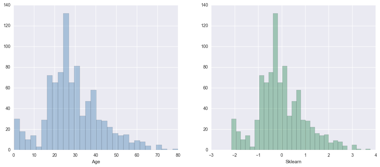
from sklearn.preprocessing import StandardScaler

std_scale = StandardScaler()
age_df_std = std_scale.fit_transform(df[['Age']])
fig, ax = plt.subplots(1,2, figsize=(15,6))
sns.distplot(df['Age'], ax=ax[0], kde=False, color="steelblue", bins=30)
sns.distplot(age_df_std, ax=ax[1], kde=False, color="seagreen", bins=30)
ax[1].set_xlabel('Sklearn');
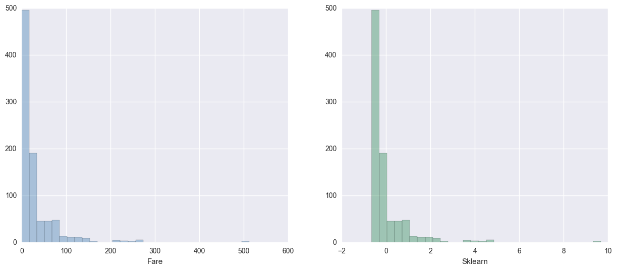
# Standardize Fare
std_scale = StandardScaler()
fare_df_std = std_scale.fit_transform(df[['Fare']])
fig, ax = plt.subplots(1,2, figsize=(15,6))
sns.distplot(df['Fare'], ax=ax[0], kde=False, color="steelblue", bins=30)
sns.distplot(fare_df_std, ax=ax[1], kde=False, color="seagreen", bins=30)
ax[1].set_xlabel('Sklearn');
|
Survived |
Pclass |
Name |
Sex |
Age |
SibSp |
Parch |
Ticket |
Fare |
Cabin |
Embarked |
Fsize |
title |
deck |
surname |
| 0 |
0 |
3 |
Braund, Mr. Owen Harris |
male |
22.0 |
1 |
0 |
A/5 21171 |
7.2500 |
X |
S |
2 |
Mr |
X |
Braund |
| 1 |
1 |
1 |
Cumings, Mrs. John Bradley (Florence Briggs Th... |
female |
38.0 |
1 |
0 |
PC 17599 |
71.2833 |
C85 |
C |
2 |
Mrs |
C |
Cumings |
| 2 |
1 |
3 |
Heikkinen, Miss. Laina |
female |
26.0 |
0 |
0 |
STON/O2. 3101282 |
7.9250 |
X |
S |
1 |
Miss |
X |
Heikkinen |
| 3 |
1 |
1 |
Futrelle, Mrs. Jacques Heath (Lily May Peel) |
female |
35.0 |
1 |
0 |
113803 |
53.1000 |
C123 |
S |
2 |
Mrs |
C |
Futrelle |
| 4 |
0 |
3 |
Allen, Mr. William Henry |
male |
35.0 |
0 |
0 |
373450 |
8.0500 |
X |
S |
1 |
Mr |
X |
Allen |
lr_drop = ['Name', 'Ticket', 'Cabin', 'surname']
df_lr.drop(lr_drop, axis=1, inplace=True)
df_lr.head()
|
Survived |
Pclass |
Sex |
Age |
SibSp |
Parch |
Fare |
Embarked |
Fsize |
title |
deck |
| 0 |
0 |
3 |
male |
22.0 |
1 |
0 |
7.2500 |
S |
2 |
Mr |
X |
| 1 |
1 |
1 |
female |
38.0 |
1 |
0 |
71.2833 |
C |
2 |
Mrs |
C |
| 2 |
1 |
3 |
female |
26.0 |
0 |
0 |
7.9250 |
S |
1 |
Miss |
X |
| 3 |
1 |
1 |
female |
35.0 |
1 |
0 |
53.1000 |
S |
2 |
Mrs |
C |
| 4 |
0 |
3 |
male |
35.0 |
0 |
0 |
8.0500 |
S |
1 |
Mr |
X |
df_lr['Sex'] = df_lr['Sex'].apply(lambda x: 1 if x == 'male' else 0)
df_lr['Survived'][df_lr['Survived'] == 0].count()*1.0/(df_lr['Survived'][df_lr['Survived'] == 0].count()+\
                                                   df_lr['Survived'][df_lr['Survived'] == 1].count())*1.0
df_lr = pd.get_dummies(df_lr)
df_lr.columns
Index([    u'Survived',       u'Pclass',          u'Sex',          u'Age',
              u'SibSp',        u'Parch',         u'Fare',        u'Fsize',
         u'Embarked_C',   u'Embarked_Q',   u'Embarked_S',     u'title_Dr',
         u'title_Lady',   u'title_MHon', u'title_Master',   u'title_Miss',
           u'title_Mr',    u'title_Mrs',     u'title_Ms',    u'title_Rev',
          u'title_Sir',       u'deck_A',       u'deck_B',       u'deck_C',
             u'deck_D',       u'deck_E',       u'deck_F',       u'deck_G',
             u'deck_T',       u'deck_X'],
      dtype='object')
df_lr.drop(['Embarked_C','title_Mr','deck_X'], axis=1, inplace=True)
df_lr.head()
|
Survived |
Pclass |
Sex |
Age |
SibSp |
Parch |
Fare |
Fsize |
Embarked_Q |
Embarked_S |
... |
title_Rev |
title_Sir |
deck_A |
deck_B |
deck_C |
deck_D |
deck_E |
deck_F |
deck_G |
deck_T |
| 0 |
0 |
3 |
1 |
22.0 |
1 |
0 |
7.2500 |
2 |
0.0 |
1.0 |
... |
0.0 |
0.0 |
0.0 |
0.0 |
0.0 |
0.0 |
0.0 |
0.0 |
0.0 |
0.0 |
| 1 |
1 |
1 |
0 |
38.0 |
1 |
0 |
71.2833 |
2 |
0.0 |
0.0 |
... |
0.0 |
0.0 |
0.0 |
0.0 |
1.0 |
0.0 |
0.0 |
0.0 |
0.0 |
0.0 |
| 2 |
1 |
3 |
0 |
26.0 |
0 |
0 |
7.9250 |
1 |
0.0 |
1.0 |
... |
0.0 |
0.0 |
0.0 |
0.0 |
0.0 |
0.0 |
0.0 |
0.0 |
0.0 |
0.0 |
| 3 |
1 |
1 |
0 |
35.0 |
1 |
0 |
53.1000 |
2 |
0.0 |
1.0 |
... |
0.0 |
0.0 |
0.0 |
0.0 |
1.0 |
0.0 |
0.0 |
0.0 |
0.0 |
0.0 |
| 4 |
0 |
3 |
1 |
35.0 |
0 |
0 |
8.0500 |
1 |
0.0 |
1.0 |
... |
0.0 |
0.0 |
0.0 |
0.0 |
0.0 |
0.0 |
0.0 |
0.0 |
0.0 |
0.0 |
5 rows × 27 columns
df_lr = pd.concat([df_lr.drop('Pclass',axis=1),pd.get_dummies(df_lr['Pclass'], prefix='Class',drop_first=True)], axis = 1)
df_lr = pd.concat([df_lr.drop('SibSp',axis=1),pd.get_dummies(df_lr['SibSp'], prefix='SibSp',drop_first=True)], axis = 1)
df_lr = pd.concat([df_lr.drop('Parch',axis=1),pd.get_dummies(df_lr['Parch'], prefix='Parch',drop_first=True)], axis = 1)
df_lr = pd.concat([df_lr.drop('Fsize',axis=1),pd.get_dummies(df_lr['Fsize'], prefix='Fsize',drop_first=True)], axis = 1)
df_lr['age_std'] = age_df_std
df_lr['fare_std'] = fare_df_std
Index([    u'Survived',          u'Sex',          u'Age',         u'Fare',
         u'Embarked_Q',   u'Embarked_S',     u'title_Dr',   u'title_Lady',
         u'title_MHon', u'title_Master',   u'title_Miss',    u'title_Mrs',
           u'title_Ms',    u'title_Rev',    u'title_Sir',       u'deck_A',
             u'deck_B',       u'deck_C',       u'deck_D',       u'deck_E',
             u'deck_F',       u'deck_G',       u'deck_T',      u'Class_2',
            u'Class_3',      u'SibSp_1',      u'SibSp_2',      u'SibSp_3',
            u'SibSp_4',      u'SibSp_5',      u'SibSp_8',      u'Parch_1',
            u'Parch_2',      u'Parch_3',      u'Parch_4',      u'Parch_5',
            u'Parch_6',      u'Fsize_2',      u'Fsize_3',      u'Fsize_4',
            u'Fsize_5',      u'Fsize_6',      u'Fsize_7',      u'Fsize_8',
           u'Fsize_11',      u'age_std',     u'fare_std'],
      dtype='object')
df_lr.drop(['Age','Fare'], axis=1, inplace=True)
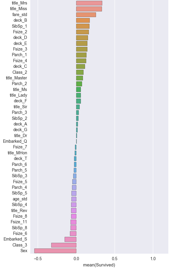
corr = df_lr.corr(method='pearson', min_periods=1).iloc[:,0]
corr = corr[np.argsort(corr, axis=0)[::-1]]
corr = pd.DataFrame(corr)
plt.figure(figsize=(6, 0.25*len(corr)))
sns.barplot(data=corr, y=corr.index, x=corr['Survived'], orient='h')
<matplotlib.axes._subplots.AxesSubplot at 0x11a133690>
X_lr = df_lr.iloc[:,1:]
y_lr = df_lr['Survived']
|
Sex |
Embarked_Q |
Embarked_S |
title_Dr |
title_Lady |
title_MHon |
title_Master |
title_Miss |
title_Mrs |
title_Ms |
... |
Fsize_2 |
Fsize_3 |
Fsize_4 |
Fsize_5 |
Fsize_6 |
Fsize_7 |
Fsize_8 |
Fsize_11 |
age_std |
fare_std |
| 0 |
1 |
0.0 |
1.0 |
0.0 |
0.0 |
0.0 |
0.0 |
0.0 |
0.0 |
0.0 |
... |
1.0 |
0.0 |
0.0 |
0.0 |
0.0 |
0.0 |
0.0 |
0.0 |
-0.529702 |
-0.502445 |
| 1 |
0 |
0.0 |
0.0 |
0.0 |
0.0 |
0.0 |
0.0 |
0.0 |
1.0 |
0.0 |
... |
1.0 |
0.0 |
0.0 |
0.0 |
0.0 |
0.0 |
0.0 |
0.0 |
0.656200 |
0.786845 |
| 2 |
0 |
0.0 |
1.0 |
0.0 |
0.0 |
0.0 |
0.0 |
1.0 |
0.0 |
0.0 |
... |
0.0 |
0.0 |
0.0 |
0.0 |
0.0 |
0.0 |
0.0 |
0.0 |
-0.233226 |
-0.488854 |
| 3 |
0 |
0.0 |
1.0 |
0.0 |
0.0 |
0.0 |
0.0 |
0.0 |
1.0 |
0.0 |
... |
1.0 |
0.0 |
0.0 |
0.0 |
0.0 |
0.0 |
0.0 |
0.0 |
0.433843 |
0.420730 |
| 4 |
1 |
0.0 |
1.0 |
0.0 |
0.0 |
0.0 |
0.0 |
0.0 |
0.0 |
0.0 |
... |
0.0 |
0.0 |
0.0 |
0.0 |
0.0 |
0.0 |
0.0 |
0.0 |
0.433843 |
-0.486337 |
5 rows × 44 columns
# Split training and test
from sklearn.model_selection import train_test_split, cross_val_score

Xlr_train, Xlr_test, ylr_train, ylr_test = train_test_split(X_lr, y_lr, test_size=.30, random_state=42)
from sklearn.linear_model import LogisticRegression
# fit model
lr = LogisticRegression()
lr_model = lr.fit(Xlr_train, ylr_train)
# predictions
ylr_pred = lr_model.predict(Xlr_test)
from sklearn.metrics import accuracy_score, confusion_matrix, classification_report

acc = accuracy_score(ylr_test, ylr_pred)
# conf matrix
lr_cm = confusion_matrix(ylr_test, ylr_pred)
lr_cm = pd.DataFrame(lr_cm, columns=["Survived-N", "Survived-Y"], index=["Survived-N", "Survived-Y"])
lr_cm
|
Survived-N |
Survived-Y |
| Survived-N |
138 |
19 |
| Survived-Y |
29 |
82 |
from sklearn.metrics import classification_report

print(classification_report(ylr_test, ylr_pred))
             precision    recall  f1-score   support

          0       0.83      0.88      0.85       157
          1       0.81      0.74      0.77       111

avg / total       0.82      0.82      0.82       268
Our recall on the positive class is only 74%. Let’s tune to see if we can improve and then think about adjusting the threshold so that we increase the recall on the positive class.
cv_lr = cross_val_score(lr, X_lr, y_lr, cv=3)
cv_lr
array([ 0.80808081, 0.82491582, 0.82154882])
{'C': 1.0,
 'class_weight': None,
 'dual': False,
 'fit_intercept': True,
 'intercept_scaling': 1,
 'max_iter': 100,
 'multi_class': 'ovr',
 'n_jobs': 1,
 'penalty': 'l2',
 'random_state': None,
 'solver': 'liblinear',
 'tol': 0.0001,
 'verbose': 0,
 'warm_start': False}
from sklearn.model_selection import GridSearchCV
lrcv = LogisticRegression(verbose=False)
Cs = [0.0001, 0.001, 0.01, 0.1, .15, .25, .275, .33, 0.5, .66, 0.75, 1.0, 2.5, 5.0, 10.0, 100.0, 1000.0]
penalties = ['l1','l2']

gs = GridSearchCV(lrcv, {'penalty': penalties, 'C': Cs},verbose=False, cv=15)
gs.fit(Xlr_train, ylr_train)
GridSearchCV(cv=15, error_score='raise',
       estimator=LogisticRegression(C=1.0, class_weight=None, dual=False, fit_intercept=True,
          intercept_scaling=1, max_iter=100, multi_class='ovr', n_jobs=1,
          penalty='l2', random_state=None, solver='liblinear', tol=0.0001,
          verbose=False, warm_start=False),
       fit_params={}, iid=True, n_jobs=1,
       param_grid={'penalty': ['l1', 'l2'], 'C': [0.0001, 0.001, 0.01, 0.1, 0.15, 0.25, 0.275, 0.33, 0.5, 0.66, 0.75, 1.0, 2.5, 5.0, 10.0, 100.0, 1000.0]},
       pre_dispatch='2*n_jobs', refit=True, return_train_score=True,
       scoring=None, verbose=False)
print gs.best_params_
print gs.best_score_
{'penalty': 'l2', 'C': 1.0}
0.841091492777
lr2 = LogisticRegression(penalty='l2', C=1.0)
lr2_model = lr2.fit(Xlr_train, ylr_train)
# predictions
ylr_pred = lr2_model.predict(Xlr_test)
acc = accuracy_score(ylr_test, ylr_pred)
acc
# conf matrix
lr_cm = confusion_matrix(ylr_test, ylr_pred)
lr_cm = pd.DataFrame(lr_cm, columns=["Survived_N", "Survived_Y"], index=["Survived_N", "Survived_Y"])
lr_cm
|
Survived_N |
Survived_Y |
| Survived_N |
138 |
19 |
| Survived_Y |
29 |
82 |
# lrcv_model.predict_proba(Xlr_test)
from sklearn.metrics import roc_curve, auc
import matplotlib.pyplot as plt
plt.style.use('seaborn-white')
%matplotlib inline

Y_score = lr2_model.decision_function(Xlr_test)

FPR = dict()
TPR = dict()
ROC_AUC = dict()

# For class 1, find the area under the curve
FPR[1], TPR[1], _ = roc_curve(ylr_test, Y_score)
ROC_AUC[1] = auc(FPR[1], TPR[1])

# Plot of a ROC curve for class 1 (has_cancer)
plt.figure(figsize=[6,5])
plt.plot(FPR[1], TPR[1], label='ROC curve (area = %0.2f)' % ROC_AUC[1], linewidth=4)
plt.plot([0, 1], [0, 1], 'k--', linewidth=4)
plt.xlim([0.0, 1.0])
plt.ylim([0.0, 1.05])
plt.xlabel('False Positive Rate', fontsize=18)
plt.ylabel('True Positive Rate', fontsize=18)
plt.title('ROC for predicting Survival', fontsize=18)
plt.legend(loc="lower right")
plt.show()
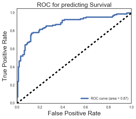
# Lets try to improve our recall on the positive class using the above roc to aim for about 86% recall.
lrcv3 = LogisticRegression(penalty='l2', C=1.0, class_weight={1: 0.95, 0:.30})
lrcv3_model = lrcv3.fit(Xlr_train, ylr_train)
# predictions
ylr_pred3 = lrcv3_model.predict(Xlr_test)
# conf matrix
lr_cm3 = confusion_matrix(ylr_test, ylr_pred3)
lr_cm3 = pd.DataFrame(lr_cm3, columns=["Survived_N", "Survived_Y"], index=["Survived_N", "Survived_Y"])
lr_cm3
|
Survived_N |
Survived_Y |
| Survived_N |
120 |
37 |
| Survived_Y |
16 |
95 |
print(classification_report(ylr_test, ylr_pred3))
             precision    recall  f1-score   support

          0       0.88      0.76      0.82       157
          1       0.72      0.86      0.78       111

avg / total       0.81      0.80      0.80       268
Lets look at Knn
# We will have to rescale our our age feature, we are going to leave out fare
# I wonder if it matters if we min max scale from standardized data.
from sklearn.preprocessing import MinMaxScaler
scaler = MinMaxScaler()
age_scaled = scaler.fit_transform(df_knn['age_std'])
df_knn['age_scaled'] = age_scaled
//anaconda/lib/python2.7/site-packages/sklearn/preprocessing/data.py:321: DeprecationWarning: Passing 1d arrays as data is deprecated in 0.17 and will raise ValueError in 0.19. Reshape your data either using X.reshape(-1, 1) if your data has a single feature or X.reshape(1, -1) if it contains a single sample.
  warnings.warn(DEPRECATION_MSG_1D, DeprecationWarning)
//anaconda/lib/python2.7/site-packages/sklearn/preprocessing/data.py:356: DeprecationWarning: Passing 1d arrays as data is deprecated in 0.17 and will raise ValueError in 0.19. Reshape your data either using X.reshape(-1, 1) if your data has a single feature or X.reshape(1, -1) if it contains a single sample.
  warnings.warn(DEPRECATION_MSG_1D, DeprecationWarning)
df_knn.drop(['age_std', 'fare_std'], axis=1, inplace=True)
df_knn.drop(['Embarked_Q', 'Embarked_S'], axis=1, inplace=True)
Index([    u'Survived',          u'Sex',     u'title_Dr',   u'title_Lady',
         u'title_MHon', u'title_Master',   u'title_Miss',    u'title_Mrs',
           u'title_Ms',    u'title_Rev',    u'title_Sir',       u'deck_A',
             u'deck_B',       u'deck_C',       u'deck_D',       u'deck_E',
             u'deck_F',       u'deck_G',       u'deck_T',      u'Class_2',
            u'Class_3',      u'SibSp_1',      u'SibSp_2',      u'SibSp_3',
            u'SibSp_4',      u'SibSp_5',      u'SibSp_8',      u'Parch_1',
            u'Parch_2',      u'Parch_3',      u'Parch_4',      u'Parch_5',
            u'Parch_6',      u'Fsize_2',      u'Fsize_3',      u'Fsize_4',
            u'Fsize_5',      u'Fsize_6',      u'Fsize_7',      u'Fsize_8',
           u'Fsize_11',   u'age_scaled'],
      dtype='object')
df_knn.drop(['deck_A','deck_B','deck_C','deck_D','deck_E','deck_F','deck_G','deck_T'], axis=1, inplace=True)
df_knn.drop(['SibSp_1','SibSp_2','SibSp_3','SibSp_4','SibSp_5','SibSp_8'], axis=1, inplace=True)
df_knn.drop(['Parch_1','Parch_2','Parch_3','Parch_4','Parch_5','Parch_6'], axis=1, inplace=True)
df_knn.drop(['title_Dr','title_Lady','title_MHon', 'title_Master','title_Miss',\
             'title_Mrs','title_Ms','title_Rev','title_Sir'], axis=1, inplace=True)
X_knn = df_knn.iloc[:,1:]
y_knn = df_knn['Survived']
|
Sex |
Class_2 |
Class_3 |
Fsize_2 |
Fsize_3 |
Fsize_4 |
Fsize_5 |
Fsize_6 |
Fsize_7 |
Fsize_8 |
Fsize_11 |
age_scaled |
| 0 |
1 |
0.0 |
1.0 |
1.0 |
0.0 |
0.0 |
0.0 |
0.0 |
0.0 |
0.0 |
0.0 |
0.271174 |
| 1 |
0 |
0.0 |
0.0 |
1.0 |
0.0 |
0.0 |
0.0 |
0.0 |
0.0 |
0.0 |
0.0 |
0.472229 |
| 2 |
0 |
0.0 |
1.0 |
0.0 |
0.0 |
0.0 |
0.0 |
0.0 |
0.0 |
0.0 |
0.0 |
0.321438 |
| 3 |
0 |
0.0 |
0.0 |
1.0 |
0.0 |
0.0 |
0.0 |
0.0 |
0.0 |
0.0 |
0.0 |
0.434531 |
| 4 |
1 |
0.0 |
1.0 |
0.0 |
0.0 |
0.0 |
0.0 |
0.0 |
0.0 |
0.0 |
0.0 |
0.434531 |
Xknn_train, Xknn_test, yknn_train, yknn_test = train_test_split(X_knn, y_knn, test_size=.30, random_state=78)
from sklearn.neighbors import KNeighborsClassifier
knn = KNeighborsClassifier(n_neighbors=3, weights='uniform')

knn.fit(Xknn_train,yknn_train)
KNeighborsClassifier(algorithm='auto', leaf_size=30, metric='minkowski',
           metric_params=None, n_jobs=1, n_neighbors=3, p=2,
           weights='uniform')
# Check accuracy
knn_pred = knn.predict(Xknn_test)
accuracy_score(yknn_test, knn_pred)
:P, Reducing our features to four categories brought our accuracy from low 70’s to 84.
# Let's gridsearch some parameters for knn
K = range(1,11)
wghts = ['uniform','distance']

knn = KNeighborsClassifier()

gs = GridSearchCV(knn, {'n_neighbors': K, 'weights':wghts}, cv=3)
gs.fit(X_knn, y_knn)
GridSearchCV(cv=3, error_score='raise',
       estimator=KNeighborsClassifier(algorithm='auto', leaf_size=30, metric='minkowski',
           metric_params=None, n_jobs=1, n_neighbors=5, p=2,
           weights='uniform'),
       fit_params={}, iid=True, n_jobs=1,
       param_grid={'n_neighbors': [1, 2, 3, 4, 5, 6, 7, 8, 9, 10], 'weights': ['uniform', 'distance']},
       pre_dispatch='2*n_jobs', refit=True, return_train_score=True,
       scoring=None, verbose=0)
print gs.best_params_
print gs.best_score_
{'n_neighbors': 4, 'weights': 'uniform'}
0.814814814815
knn = KNeighborsClassifier(n_neighbors=4, weights='uniform')

knn.fit(Xknn_train,yknn_train)
KNeighborsClassifier(algorithm='auto', leaf_size=30, metric='minkowski',
           metric_params=None, n_jobs=1, n_neighbors=4, p=2,
           weights='uniform')
# Check accuracy
knn_pred = knn.predict(Xknn_test)
accuracy_score(yknn_test, knn_pred)
after tuning our model with gridsearch we get a slightly lower accuracy score, possibly due to the fold size and split of the data.
# conf matrix
knn_cm = confusion_matrix(yknn_test, knn_pred)
knn_cm = pd.DataFrame(knn_cm, columns=["Survived_N", "Survived_Y"], index=["Survived_N", "Survived_Y"])
knn_cm
|
Survived_N |
Survived_Y |
| Survived_N |
153 |
13 |
| Survived_Y |
37 |
65 |
print(classification_report(yknn_test, knn_pred))
             precision    recall  f1-score   support

          0       0.81      0.92      0.86       166
          1       0.83      0.64      0.72       102

avg / total       0.82      0.81      0.81       268
Y_score = knn.predict_proba(Xknn_test)[:,1]


FPR = dict()
TPR = dict()
ROC_AUC = dict()

# For class 1, find the area under the curve
FPR[1], TPR[1], _ = roc_curve(yknn_test, Y_score)
ROC_AUC[1] = auc(FPR[1], TPR[1])

# Plot of a ROC curve for class 1 (has_cancer)
plt.figure(figsize=[6,5])
plt.plot(FPR[1], TPR[1], label='ROC curve (area = %0.2f)' % ROC_AUC[1], linewidth=4)
plt.plot([0, 1], [0, 1], 'k--', linewidth=4)
plt.xlim([0.0, 1.0])
plt.ylim([0.0, 1.05])
plt.xlabel('False Positive Rate', fontsize=18)
plt.ylabel('True Positive Rate', fontsize=18)
plt.title('Knn - ROC for predicting Survival', fontsize=18)
plt.legend(loc="lower right")
plt.show()
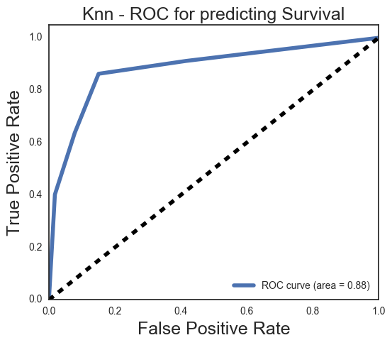
# knn does better capturing non-survivors with a 92% recall, but is worse on survivors with a recall of 64,
# while maintaining a similar accuaracy as log reg
# Lets try a decision tree
from sklearn.tree import DecisionTreeClassifier
to_drop = ['Name', 'Ticket', 'Cabin', 'surname']
df_tree.drop(to_drop, axis=1, inplace=True)
df_tree.head()
|
Survived |
Pclass |
Sex |
Age |
SibSp |
Parch |
Fare |
Embarked |
Fsize |
title |
deck |
| 0 |
0 |
3 |
male |
22.0 |
1 |
0 |
7.2500 |
S |
2 |
Mr |
X |
| 1 |
1 |
1 |
female |
38.0 |
1 |
0 |
71.2833 |
C |
2 |
Mrs |
C |
| 2 |
1 |
3 |
female |
26.0 |
0 |
0 |
7.9250 |
S |
1 |
Miss |
X |
| 3 |
1 |
1 |
female |
35.0 |
1 |
0 |
53.1000 |
S |
2 |
Mrs |
C |
| 4 |
0 |
3 |
male |
35.0 |
0 |
0 |
8.0500 |
S |
1 |
Mr |
X |
df_tree['Sex'] = df_tree['Sex'].apply(lambda x: 1 if x == 'male' else 0)
df_tree = pd.concat([df_tree.drop('Pclass',axis=1),pd.get_dummies(df['Pclass'], prefix='Class')], axis = 1)
df_tree = pd.concat([df_tree.drop('Fsize',axis=1),pd.get_dummies(df['Fsize'], prefix='Fsize')], axis = 1)
ytr = df_tree['Survived']
Xtr = pd.get_dummies(df_tree.drop('Survived', axis=1))
Xtr.head()
|
Sex |
Age |
SibSp |
Parch |
Fare |
Class_1 |
Class_2 |
Class_3 |
Fsize_1 |
Fsize_2 |
... |
title_Sir |
deck_A |
deck_B |
deck_C |
deck_D |
deck_E |
deck_F |
deck_G |
deck_T |
deck_X |
| 0 |
1 |
22.0 |
1 |
0 |
7.2500 |
0.0 |
0.0 |
1.0 |
0.0 |
1.0 |
... |
0.0 |
0.0 |
0.0 |
0.0 |
0.0 |
0.0 |
0.0 |
0.0 |
0.0 |
1.0 |
| 1 |
0 |
38.0 |
1 |
0 |
71.2833 |
1.0 |
0.0 |
0.0 |
0.0 |
1.0 |
... |
0.0 |
0.0 |
0.0 |
1.0 |
0.0 |
0.0 |
0.0 |
0.0 |
0.0 |
0.0 |
| 2 |
0 |
26.0 |
0 |
0 |
7.9250 |
0.0 |
0.0 |
1.0 |
1.0 |
0.0 |
... |
0.0 |
0.0 |
0.0 |
0.0 |
0.0 |
0.0 |
0.0 |
0.0 |
0.0 |
1.0 |
| 3 |
0 |
35.0 |
1 |
0 |
53.1000 |
1.0 |
0.0 |
0.0 |
0.0 |
1.0 |
... |
0.0 |
0.0 |
0.0 |
1.0 |
0.0 |
0.0 |
0.0 |
0.0 |
0.0 |
0.0 |
| 4 |
1 |
35.0 |
0 |
0 |
8.0500 |
0.0 |
0.0 |
1.0 |
1.0 |
0.0 |
... |
0.0 |
0.0 |
0.0 |
0.0 |
0.0 |
0.0 |
0.0 |
0.0 |
0.0 |
1.0 |
5 rows × 39 columns
Xtr_train, Xtr_test, ytr_train, ytr_test = train_test_split(Xtr, ytr, test_size=.30, random_state=42)
dt = DecisionTreeClassifier(max_depth = 20)

dt.fit(Xtr_train, ytr_train)
DecisionTreeClassifier(class_weight=None, criterion='gini', max_depth=20,
            max_features=None, max_leaf_nodes=None,
            min_impurity_split=1e-07, min_samples_leaf=1,
            min_samples_split=2, min_weight_fraction_leaf=0.0,
            presort=False, random_state=None, splitter='best')
feature_importances = pd.DataFrame(dt.feature_importances_,
                                   index = Xtr_train.columns,
                                    columns=['importance'])
feature_importances.sort_values(by='importance', ascending=False)
|
importance |
| title_Mr |
0.301381 |
| Fare |
0.265834 |
| Age |
0.140920 |
| Class_3 |
0.093943 |
| title_Rev |
0.024041 |
| Parch |
0.019571 |
| deck_E |
0.017983 |
| Embarked_S |
0.015582 |
| deck_B |
0.015014 |
| title_Dr |
0.013680 |
| Embarked_C |
0.012709 |
| Fsize_4 |
0.011801 |
| Fsize_5 |
0.008725 |
| deck_X |
0.008162 |
| deck_C |
0.007443 |
| Embarked_Q |
0.006782 |
| Fsize_2 |
0.006149 |
| Class_2 |
0.005454 |
| SibSp |
0.004794 |
| deck_D |
0.004494 |
| Fsize_7 |
0.003923 |
| deck_T |
0.003596 |
| Fsize_1 |
0.003596 |
| Class_1 |
0.002865 |
| Fsize_3 |
0.001557 |
| title_Sir |
0.000000 |
| deck_G |
0.000000 |
| deck_F |
0.000000 |
| deck_A |
0.000000 |
| title_Mrs |
0.000000 |
| title_Ms |
0.000000 |
| Fsize_8 |
0.000000 |
| title_Miss |
0.000000 |
| title_Master |
0.000000 |
| title_MHon |
0.000000 |
| title_Lady |
0.000000 |
| Fsize_6 |
0.000000 |
| Fsize_11 |
0.000000 |
| Sex |
0.000000 |
# Check accuracy
dt_pred = dt.predict(Xtr_test)
accuracy_score(ytr_test, dt_pred)
K = range(5,31)
wghts = ['balanced', None]

dt = DecisionTreeClassifier()

gs = GridSearchCV(dt, {'max_depth': K, 'class_weight':wghts}, cv=15)
gs.fit(Xtr, ytr)
GridSearchCV(cv=15, error_score='raise',
       estimator=DecisionTreeClassifier(class_weight=None, criterion='gini', max_depth=None,
            max_features=None, max_leaf_nodes=None,
            min_impurity_split=1e-07, min_samples_leaf=1,
            min_samples_split=2, min_weight_fraction_leaf=0.0,
            presort=False, random_state=None, splitter='best'),
       fit_params={}, iid=True, n_jobs=1,
       param_grid={'max_depth': [5, 6, 7, 8, 9, 10, 11, 12, 13, 14, 15, 16, 17, 18, 19, 20, 21, 22, 23, 24, 25, 26, 27, 28, 29, 30], 'class_weight': ['balanced', None]},
       pre_dispatch='2*n_jobs', refit=True, return_train_score=True,
       scoring=None, verbose=0)
print gs.best_params_
print gs.best_score_
{'max_depth': 8, 'class_weight': None}
0.81593714927
# re fit model with max depth 8
dt = DecisionTreeClassifier(max_depth = 8)

dt.fit(Xtr_train, ytr_train)
DecisionTreeClassifier(class_weight=None, criterion='gini', max_depth=8,
            max_features=None, max_leaf_nodes=None,
            min_impurity_split=1e-07, min_samples_leaf=1,
            min_samples_split=2, min_weight_fraction_leaf=0.0,
            presort=False, random_state=None, splitter='best')
# Check accuracy
dt_pred = dt.predict(Xtr_test)
accuracy_score(ytr_test, dt_pred)
# get a slightly better acuuracy than before gridsearch
# conf matrix
dt_cm = confusion_matrix(ytr_test, dt_pred)
dt_cm = pd.DataFrame(dt_cm, columns=["Survived_N", "Survived_Y"], index=["Survived_N", "Survived_Y"])
dt_cm
|
Survived_N |
Survived_Y |
| Survived_N |
136 |
21 |
| Survived_Y |
29 |
82 |
# looks pretty much the same as the first logistic regression
# predicted 82 survivors correctly, but missed 29 survivors and also classified 19 non-survivors as survivors.
print(classification_report(ytr_test, dt_pred))
             precision    recall  f1-score   support

          0       0.82      0.87      0.84       157
          1       0.80      0.74      0.77       111

avg / total       0.81      0.81      0.81       268
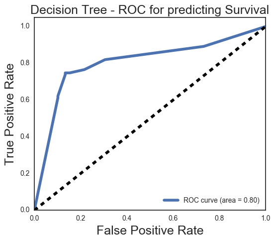
# Our precision is fairly good, but our recall on class 1 - survival - is a bit lower,
# missing 26% of of survivors (29)
Y_score = dt.predict_proba(Xtr_test)[:,1]


FPR = dict()
TPR = dict()
ROC_AUC = dict()

# For class 1, find the area under the curve
FPR[1], TPR[1], _ = roc_curve(ytr_test, Y_score)
ROC_AUC[1] = auc(FPR[1], TPR[1])

# Plot of a ROC curve for class 1 (has_cancer)
plt.figure(figsize=[6,5])
plt.plot(FPR[1], TPR[1], label='ROC curve (area = %0.2f)' % ROC_AUC[1], linewidth=4)
plt.plot([0, 1], [0, 1], 'k--', linewidth=4)
plt.xlim([0.0, 1.0])
plt.ylim([0.0, 1.05])
plt.xlabel('False Positive Rate', fontsize=18)
plt.ylabel('True Positive Rate', fontsize=18)
plt.title('Decision Tree - ROC for predicting Survival', fontsize=18)
plt.legend(loc="lower right")
plt.show()
# Lets adjust the decision threshold
dt2 = DecisionTreeClassifier(max_depth = 8, class_weight={1: 0.1, 0:.9})

dt2.fit(Xtr_train, ytr_train)
DecisionTreeClassifier(class_weight={0: 0.9, 1: 0.1}, criterion='gini',
            max_depth=8, max_features=None, max_leaf_nodes=None,
            min_impurity_split=1e-07, min_samples_leaf=1,
            min_samples_split=2, min_weight_fraction_leaf=0.0,
            presort=False, random_state=None, splitter='best')
dt2_pred = dt2.predict(Xtr_test)
accuracy_score(ytr_test, dt2_pred)
# conf matrix
dt2_cm = confusion_matrix(ytr_test, dt2_pred)
dt2_cm = pd.DataFrame(dt2_cm, columns=["P_Survived_N", "P_Survived_Y"], index=["Survived_N", "Survived_Y"])
dt2_cm
|
P_Survived_N |
P_Survived_Y |
| Survived_N |
147 |
10 |
| Survived_Y |
48 |
63 |
|
Survived_N |
Survived_Y |
| Survived_N |
136 |
21 |
| Survived_Y |
29 |
82 |
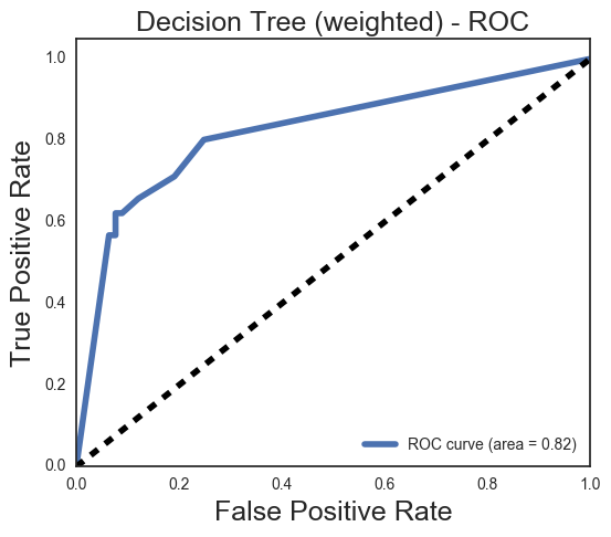
We increased the weight of the non-survivor class to be able to identify more people
who would likely be at risk in a disastor. The recall on our 0 class is bumped up without too much sacrifice to accuracy.
print(classification_report(ytr_test, dt2_pred))
             precision    recall  f1-score   support

          0       0.75      0.94      0.84       157
          1       0.86      0.57      0.68       111

avg / total       0.80      0.78      0.77       268
Y_score = dt2.predict_proba(Xtr_test)[:,1]


FPR = dict()
TPR = dict()
ROC_AUC = dict()

# For class 1, find the area under the curve
FPR[1], TPR[1], _ = roc_curve(ytr_test, Y_score)
ROC_AUC[1] = auc(FPR[1], TPR[1])

# Plot of a ROC curve for class 1 (has_cancer)
plt.figure(figsize=[6,5])
plt.plot(FPR[1], TPR[1], label='ROC curve (area = %0.2f)' % ROC_AUC[1], linewidth=4)
plt.plot([0, 1], [0, 1], 'k--', linewidth=4)
plt.xlim([0.0, 1.0])
plt.ylim([0.0, 1.05])
plt.xlabel('False Positive Rate', fontsize=18)
plt.ylabel('True Positive Rate', fontsize=18)
plt.title('Decision Tree (weighted) - ROC', fontsize=18)
plt.legend(loc="lower right")
plt.show()
Y_score = dt2.predict_proba(Xtr_test)[:,1]

FPR = dict()
TPR = dict()
ROC_AUC = dict()

# For class 1, find the area under the curve
FPR[1], TPR[1], _ = roc_curve(ytr_test, Y_score)
ROC_AUC[1] = auc(FPR[1], TPR[1])

# Plot of a ROC curve for class 1 - survival
plt.subplots(figsize=(6,6));
plt.plot(FPR[1], TPR[1], label='CART ROC curve (area = %0.2f)' % ROC_AUC[1], linewidth=4)
plt.plot([0, 1], [0, 1], 'k--', linewidth=4)
plt.xlim([0.0, 1.0])
plt.ylim([0.0, 1.05])
plt.xlabel('False Positive Rate', fontsize=18)
plt.ylabel('True Positive Rate', fontsize=18)
plt.title('Predicting Survival - ROC', fontsize=18)
plt.legend(loc="lower right")

Y_score = knn.predict_proba(Xknn_test)[:,1]

FPR = dict()
TPR = dict()
ROC_AUC = dict()

FPR[1], TPR[1], _ = roc_curve(yknn_test, Y_score)
ROC_AUC[1] = auc(FPR[1], TPR[1])

plt.plot(FPR[1], TPR[1], label='Knn ROC curve (area = %0.2f)' % ROC_AUC[1], linewidth=4)
plt.plot([0, 1], [0, 1], 'k--', linewidth=4)
plt.xlim([0.0, 1.0])
plt.ylim([0.0, 1.05])
plt.xlabel('False Positive Rate', fontsize=18)
plt.ylabel('True Positive Rate', fontsize=18)
plt.legend(loc="lower right")

Y_score = lr2_model.decision_function(Xlr_test)

FPR = dict()
TPR = dict()
ROC_AUC = dict()

FPR[1], TPR[1], _ = roc_curve(ylr_test, Y_score)
ROC_AUC[1] = auc(FPR[1], TPR[1])

plt.plot(FPR[1], TPR[1], label='LR ROC curve (area = %0.2f)' % ROC_AUC[1], linewidth=4)
plt.plot([0, 1], [0, 1], 'k--', linewidth=4)
plt.xlim([0.0, 1.0])
plt.ylim([0.0, 1.05])
plt.xlabel('False Positive Rate', fontsize=18)
plt.ylabel('True Positive Rate', fontsize=18)
plt.legend(loc="lower right")
plt.show()
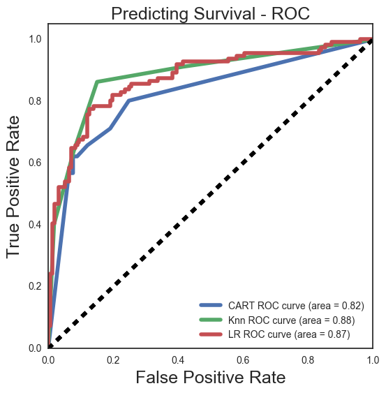
Comparing our ROC curves it looks like we can get a good tradeoff with Knn at a true positive rate of about .85 and a false positive rate of about .15
# Lets try bagging

from sklearn.ensemble import BaggingClassifier
bagger = BaggingClassifier(dt2, max_samples=1.0)

print "DT Score:\t", cross_val_score(dt2, Xtr, ytr, cv=10, n_jobs=1).mean()
print "Bagging Score:\t", cross_val_score(bagger, Xtr, ytr, cv=10, n_jobs=1).mean()
DT Score:	0.794676256952
Bagging Score:	0.811594313926
baggerk = BaggingClassifier(knn)

print "Knn Score:\t", cross_val_score(knn, X_knn, y_knn, cv=10, n_jobs=1).mean()
print "Bagging Score:\t", cross_val_score(baggerk, X_knn, y_knn, cv=10, n_jobs=1).mean()
Knn Score:	0.814951481103
Bagging Score:	0.810470434684
bagger_lr = BaggingClassifier(lr)

print "LR Score:\t", cross_val_score(lr, X_lr, y_lr, cv=10, n_jobs=1).mean()
print "Bagging Score:\t", cross_val_score(bagger_lr, X_lr, y_lr, cv=10, n_jobs=1).mean()
LR Score:	0.832780331404
Bagging Score:	0.832780331404
# Our decision tree is the only model that benefits from bagging here and only slightly.
# It perhaps was mildly overfit, while the other two were tuned fairly well already
Report
There was not much difference between each of the classifiers in this case, with just over 80% accuracy for each tuned model. Our Knn model did show a difference in the confusion matrix, having a higher recall for the non-surviving class and a lower recall on the surviving class. Knn predictions captured almost all of the non-survivors but did not capture a high amount of the surviving class.
By adjusting the class weight for a couple of models we were able to slightly increase recall on both the positive and negative class without a big decrease in accuracy. Depending on the implementation and timing one class can be weighted higher than the other to more fully identify either those at risk or those likely to survive.
Bagging only improved our decision tree model and then only slightly.
